Variable Primary Chilled Water Systems Part 2: The Darker Side of Primary Secondary Flow
/By Chad Edmondson
There are many advantages to the traditional primary secondary chilled water design, overall simplicity being at the top of the list. So why has the industry leaned into variable primary as an alternate approach over the last two decades?
Since primary secondary systems are comprised of the primary loop which flows through the chillers and the secondary loop serving the system load, there are three possible flow conditions that can occur. The primary flow can be greater than, less than, or equal to the secondary flow. The latter is the ideal condition because it keeps the two loops operating independently of one another, i.e. there is no flow in the common pipe. Unfortunately, this condition hardly ever occurs since loads are constantly changing. (See this article for a detailed explanation of the common pipe in a primary secondary system). It is the disparity of flow between the primary and secondary loops that always creates some degree of inefficiency – and in some cases extreme inefficiency.
Most of the time, primary secondary systems operate under conditions in which the primary flow is greater than the secondary flow, as shown in Figure 1. (Note that the design for this system and other examples in this blog are all the same: Two chillers at 500 tons each, 44°F chilled water supply, 56°F chilled water return, thus a 12 degree delta T, and two 1000 GPM chiller pumps.) Here we see that our system is demanding 1500 gpm of flow, so we have to turn on both chillers and primary pumps since this is a standard staged primary loop (no variable speed drives).
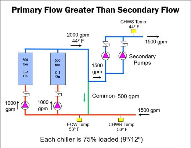
Figure 1
The chillers are partially loaded at 75% each, and we now have 2000 GPM in our primary loop even though the secondary loop is only calling for 1500 GPM. Where does that extra 500 GPM of 44°F water go? It mixes with the return 56°F water from the secondary loop and goes back to the chiller at 53°F. Obviously, there is an energy penalty associated with the extra flow through the primary loop and a lower entering chilled water return temperature to the chillers, but at least the load is satisfied.
When Secondary Flow Exceeds Primary Flow
A potentially more serious problem occurs when the primary flow is less than the secondary flow. Let’s say we have one chiller on with 1000 GPM in the primary loop at our design supply of 44°F. Our load starts to increase beyond a single chiller capacity and the system is demanding 1200 GPM from the secondary loop. Now, when that 1200 GPM of return water hits the tee on the return side of the common pipe, 200 GPM of 56°F return water will get pulled back into the supply side of the secondary loop. That means that the 56°F return water will begin mixing with the 44°F supply, increasing the supply temperature to 46°F.
If we continue to operate under these conditions, we will require a second chiller to manage the load (Figure 2).

Figure 2: When we turned on primary pump #2, the primary flow increased to 2000 GPM, but secondary flow remained at 1200 GPM.
This doubles the flow in the primary loop, but keep in mind that the secondary loop is still only flowing 1200 GPM. Now we have 800 GPM of 44°F water flowing straight through the common pipe and mixing with the 56°F return chilled water, giving us an entering temperature of 51°F to our chillers and a 7 degree delta T across our chillers. Everyone is still comfortable in the building, but the chillers are not operating as efficiently with the lower delta T because of the mixing in the common pipe.
Now let’s look at the example in Figure 3. What if our return water temperature drops to 54°F, as a result of any number of common reasons such as poor balancing, dirty coils, low control valve authority, etc.? Remember the system was designed for a 12 degree delta T but now we are only getting a 10 degree delta T. The system is demanding 500 tons of cooling, so the flow rate increases to 1200 GPM. This is just one example of the problem known as “low delta T syndrome.” In this example we must bring on a second chiller even though our load is still just 500 tons. As a result of our reduced delta T, plus the mixing of water from our chiller supply water with our return water, we are having to operate two chillers at a 6 degree delta T instead of a single chiller at a 12 degree delta T.

Figure 3

Just how much waste is associated with above scenario?
• Our primary pump brake horsepower (BHP) is over twice what it would be with a 12 degree delta T
• We are pumping 20% more flow on secondary side. Secondary pump BHP suffers an increase of approximately 60%.
• We are running two chillers instead of one; two towers instead of one; and two condenser pumps instead of one.
In addition to the energy waste and excessive wear and tear on equipment, we now have no chance whatsoever of meeting a design load of 1000 tons. If you’ve ever wondered why variable primary has become increasingly the popular, you now have your answer.
There are a few things we can do to improve the above situations without a variable primary conversion (See sidebar). But if you design chilled water systems, you need to understand the long term advantages of variable primary over constant speed primary, variable speed secondary for chilled water systems. The only exception would be a variable speed primary, variable speed secondary arrangement which would alleviate a lot of these issues. Stay tuned for more.