Fundamentals of Differential Pressure Sensored Control in Variable Speed Pumping
/By Chad Edmondson
What happens when demand drops in a closed loop variable speed system? What is the operational sequence and what logic does the controller use to vary the speed of the pump?
Let’s begin our discussion with the following system example:

Admittedly, most systems have more than one coil and pump, but this simple example will help us introduce the fundamental concept of differential pressure control, which is an essential part of variable speed pump control.
In our example, we have a design flow of 1000 GPM and 80 feet (40’ + 40’) of variable piping head loss, plus 20 feet of control head. As we learned in our last blog, control head, also referred to as “constant head,” is the minimum pump head we will have at all times. Even at zero flow, the system must be delivering this much head.
Notice that a pressure sensor is located to sense the differential pressure across the supply side of the coil and immediately after the two-way valve on the other side of the coil. The differential pressure sensor is wired into the variable speed pump control. In a differential pressure controlled system, we use these components to make sure our control head stays at its setpoint which in this case is 20 feet.
At full design conditions, we have 1000 GPM at 100 feet of head (40’+40’+20’). But what happens as demand begins to drop in this system?
The operational sequence for a system that uses sensored DP control to vary the speed of the pump is as follows:
- As demand drops, the control valve starts to close
- The closure of the control valve causes system flow to drop
- As the control valve closes, the DP sensor recognizes an increased pressure differential across the coil and control valve
- This increase in pressure differential prompts the pump controller to slow the pump speed down
- The pump slows down until the control differential pressure (20 feet in this example) is restored
Where’s the Logic?
What logic does the pump controller rely on to regulate the speed?
It’s all math, of course, and goes back to the pump affinity laws. Specifically, if you cut the flow in half, you reduce the variable head loss by a factor of 4. So, using our design coordinates of 1000 GPM and 100 feet of head as our starting point, every other operational point for the pump can be calculated. That’s where the System Syzer comes in as a handy tool, but we can also do the calculations manual and plot a system control curve.
So, in our example, if flow drops from 1000 gpm to 500 gpm, then our system head loss drops from 100 feet to 40 feet.
Still not sure where those numbers come from? Check out the figure below. If our piping loss on either side of the coil was 40 feet at 1000 GPM, then at 500 GPM, our head would drop to one quarter of 40 feet, or 10 feet of head on either side of the coil.
That is our variable head loss. Remember, we must maintain a pressure differential of 20 feet across the coil and control valve (due to the differential pressure sensor location). 10 + 20 + 10 equals 40 feet of head. At half flow we have a system head loss of 40 feet.
Using the same formula, we (or better yet, the System Syzer) can calculate the rest of the coordinates, which we can use to plot the following control curve:

Notice that at 0 flow we still have 20 feet of head!
Next week we’ll look at how changes in load impact the control curve in a more complex system.